Information on ASCENT controls

Morphology Input Files

Each mask must be binary (i.e., white pixels (‘1’) for the segmented tissue and black pixels (‘0’) elsewhere) and must use Tagged Image File Format (i.e., .tif, or .tiff).

Note

For more information on segmentation methods, see [Pelot et al., 2020]. Segmentation (i.e., marking of morphological boundaries) can be performed with paid softwares (e.g., NIS Elements, Adobe Photoshop) as well as free software (e.g., ImageJ, Gimp).

All masks must be defined within the same field of view, be the same size, and be the same resolution. To convert between pixels of the input masks to dimensioned length (micrometers), the user must specify a "ScaleInputMode" in Sample (JSON Configuration Files). If using the mask input mode, a mask for the scale bar (s.tif) of known length (oriented horizontally) must be provided (see “Scale Bar” in Fig 2) and the length of the scale bar must be indicated in Sample (JSON Configuration Files). If using the ratio input mode, the user explicitly specifies the micrometers/pixel of the input masks in Sample (JSON Configuration Files), and no scale bar image is required.

The user is required to set the "MaskInputMode" in Sample ("mask_input") to communicate the contents of the segmented histology files (JSON Configuration Files). Ideally, segmented images of boundaries for both the “outers” (o.tif) and “inners” (i.tif) of the perineurium will be provided, either as two separate files (o.tif and i.tif) or combined in the same image (c.tif) (see “Inners”, “Outers”, and “Combined” in Fig 2). However, if only inners are provided—which identify the outer edge of the endoneurium—a surrounding perineurium thickness is defined by the "PerineuriumThicknessMode" in Sample ("ci_perineurium_thickness"); the thickness is user-defined, relating perineurium thickness to features of the inners (e.g., their diameter). It should be noted that defining nerve morphology with only inners does not allow the model to represent accurately fascicles containing multiple endoneurium inners within a single outer perineurium boundary (“peanut” fascicles; see an example in Fig 2); in this case, each inner trace will be assumed to represent a single independent fascicle that does not share its perineurium with any other inners; more accurate representation requires segmentation of the “outers” as well.

The user is required to set the "NerveMode" in Sample (“nerve”) to communicate the contents of the segmented histology files (JSON Configuration Files). The outer nerve boundary, if present, is defined with a separate mask (n.tif). In the case of a compound nerve with epineurium, the pipeline expects the outer boundary of the epineurium to be provided as the “nerve”. In the case of a nerve with a single fascicle, no nerve mask is required—in which case either the outer perineurium boundary (if present) or the inner perineurium boundary (otherwise) is used as the nerve boundary—although one may be provided if epineurium or other tissue that would be within the cuff is present in the sample histology.

Lastly, an “orientation” mask (a.tif) can be optionally defined. This mask should be all black except for a small portion that is white, representing the position to which the cuff must be rotated. The angle is measured relative to the centroid of the nerve/singular fascicle, so this image should be constructed while referencing n.tif (or, if monofascicular, i.tif, o.tif, or c.tif). By default, the 0º position of our cuffs correspond with the coordinate halfway along the arc length of the cuff inner diameter (i.e., the cuff will be rotated such that the sample center, cuff contact center, and centroid of the white portion of a.tif form a line) while the circular portion of a cuff’s diameter is centered at the origin (Note: this rotation process uses "angle_to_contacts_deg" and "fixed_point" in a “preset” cuff’s JSON file, see Creating Custom Cuffs and Cuff Placement on the Nerve). If a.tif is provided, other cuff rotation methods ("cuff_shift" in Model, which calculate "pos_ang") are overridden.

The user must provide segmented image morphology files, either from histology or the mock_morphology_generator.py script, with a specific naming convention in the input/ directory.

• Raw RGB image, to be available for convenience and used for data visualization: r.tif (optional).

• Combined (i.e., inners and outers): c.tif.

• Inners: i.tif

  • An “inner” is the internal boundary of the perineurium that forms the boundary between the perineurium and the endoneurium.

• Outers: o.tif

  • An “outer” is the external boundary of the perineurium that forms the boundary between the perineurium and the epineurium or extraneural medium.

• Scale bar: s.tif (scale bar oriented horizontally, required unless scale input mode is set to ratio).

• Nerve: n.tif (optional for monofascicular nerves).

• Orientation: a.tif (optional).

For an example of input files, see Fig 2. The user must properly set the "MaskInputMode" in Sample ("mask_input") for their provided segmented image morphology files (JSON Configuration Files).

Control of medium surrounding nerve and cuff electrode

The medium surrounding the nerve and cuff electrode (e.g., fat, skeletal muscle) must contain a “proximal” domain, which runs the full length of the nerve, and may optionally include a “distal” domain. The parameterization for the geometry of the “proximal” and “distal” domains is shown below. For details on how to define the “proximal” and “distal” domain geometries and meshing parameters, see Model Parameters.

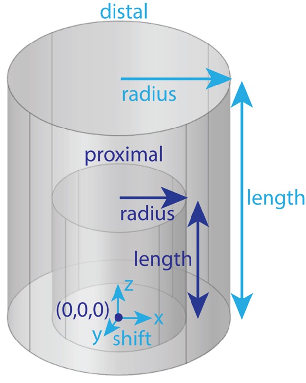
The user must define a “proximal” domain, and may optionally define a “distal” domain for independent assignment of meshing parameters for the site of stimulation from the rest of the FEM. The “proximal” domain runs the full length of the nerve and is anchored at (0,0,0). The distal domain’s radius and length may be independently assigned, and the entire distal domain may be shifted (“shift”: (x, y, z)). Having a proximal domain that is overly voluminous can significantly decrease COMSOL meshing efficiency and even, rarely, cause errors. At all costs, avoid having a proximal or distal domain whose boundary intersects with a geometry (other than the nerve ends, which are by definition at the longitudinal boundaries of the proximal domain) or the boundary of other geometries (e.g., the cuff-nerve boundary); this will likely create a meshing error.

Cuff placement on nerve

This section provides an overview of how the cuff is placed on the nerve. The compute_cuff_shift() method within Runner (src/runner.py) determines the cuff’s rotation around the nerve and translation in the (x,y)-plane. The pipeline imports the coordinates of the traces for the nerve tissue boundaries saved in samples/<sample_index>/slides/0/0/sectionwise2d/ which are, by convention, shifted such that the centroid of the nerve is at the origin (0,0) (i.e., nerve centroid from best-fit ellipse if nerve trace (n.tif) is provided, inner or outer best-fit ellipse centroid for monofascicular nerves without nerve trace). Importantly, the nerve sample cross-section is never moved from or rotated around the origin in COMSOL. By maintaining consistent nerve location across all Model’s for a Sample, the coordinates in fibersets/ are correct for any orientation of a cuff on the nerve.

ASCENT has different CuffShiftModes (i.e., "cuff_shift" parameter in Model) that control the translation of the cuff (i.e., “shift” JSON Object in Model) and default rotation around the nerve (i.e., "pos_ang" in Model). Runner’s compute_cuff_shift() method is easily expandable for users to add their own CuffShiftModes to control cuff placement on the nerve.

The rotation and translation of the cuff are populated automatically by the compute_cuff_shift() method based on sample morphology, parameterization of the “preset” cuff, and the CuffShiftMode, and are defined in the “cuff” JSON Object (“shift” and “rotate”) in Model.

For “naïve” CuffShiftModes (i.e., "NAIVE_ROTATION_MIN_CIRCLE_BOUNDARY", "NAIVE_ROTATION_TRACE_BOUNDARY") the cuff is placed on the nerve with rotation according to the parameters used to instantiate the cuff from part primitives (Part Primitives and Custom Cuffs). If the user would like to rotate the cuff from beyond this position, they may set the "add_ang" parameter in Model (Model Parameters). For naïve CuffShiftModes, the cuff is shifted along the vector from (0,0) in the direction of the "angle_to_contacts_deg" parameter in the “preset” JSON file. "NAIVE_ROTATION_MIN_CIRCLE_BOUNDARY" CuffShiftMode moves the cuff toward the nerve until the nerve’s minimum radius enclosing circle is within the distance of the "thk_medium_gap_internal" parameter for the cuff. "NAIVE_ROTATION_TRACE_BOUNDARY" CuffShiftMode moves the cuff toward the nerve until the nerve’s outermost Trace (i.e., for monofascicular nerve an inner or outer, and same result as "NAIVE_ROTATION_MIN_CIRCLE_BOUNDARY" for nerve’s with epineurium) is within the distance of the "thk_medium_gap_internal" parameter for the cuff. Note: orientation masks (a.tif) are ignored when using these modes.

For “automatic” CuffShiftModes (i.e., "AUTO_ROTATION_MIN_CIRCLE_BOUNDARY", "AUTO_ROTATION_TRACE_BOUNDARY") the cuff is rotated around the nerve based on the size and position of the nerve’s fascicle(s) before the cuff is moved toward the nerve sample (see image below). The point at the intersection of the vector from (0,0) in the direction of the "angle_to_contacts_deg" parameter in the “preset” JSON file with the cuff (i.e., cuff’s “center” in following text) is rotated to meet a specific location of the nerve/monofascicle’s surface. Specifically, the center of the cuff is rotated around the nerve to make (0,0), the center of the cuff, and Sample’s "fascicle_centroid" (computed with Slide’s fascicle_centroid() method, which calculates the area and centroid of each inner and then averages the inners’ centroids weighted by each inner’s area) colinear. If the user would like to rotate the cuff from beyond this position, they may set the "add_ang" parameter in Model (Model Parameters). The user may override the default “AUTO” rotation of the cuff on the nerve by adding an orientation mask (a.tif) to align a certain surface of the nerve sample with the cuff’s center (../Running_ASCENT/Info.md#morphology-Input-Files)). This behavior depends on the cuff’s "fixed_point" parameter (Creating Custom Cuffs) The "AUTO_ROTATION_MIN_CIRCLE_BOUNDARY" CuffShiftMode moves the cuff toward the nerve until the nerve’s minimum radius enclosing circle is within the distance of the "thk_medium_gap_internal" parameter for the cuff. "AUTO_ROTATION_TRACE_BOUNDARY" CuffShiftMode moves the cuff toward the nerve until the nerve’s outermost Trace (i.e., for monofascicular nerve an inner or outer, and same result as "AUTO_ROTATION_MIN_CIRCLE_BOUNDARY" for nerve’s with epineurium) is within the distance of the "thk_medium_gap_internal" parameter for the cuff.

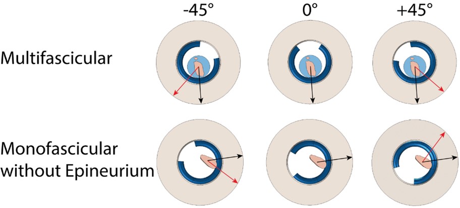
Demonstration of cuff placement on a multifascicular nerve (top) and a monofascicular nerve without epineurium (bottom) with the same “preset” cuff (Purdue.json) for three different cuff rotations using the "AUTO_ROTATION_TRACE_BOUNDARY" CuffShiftMode. The cuff rotations are different in the top and bottom rows since the point on the surface of the nerve sample closest to the most endoneurium is unique to each sample (black arrows). Additional angles of rotation were applied to the cuff directly using the “add_ang” parameter in the Model’s “cuff” JSON Object (red arrows).

The default z-position of each part along the nerve is defined in the “preset” cuff JSON file by the expression assigned to the part instance’s “Center” parameter (referenced to z = 0 at one end of the model’s proximal cylindrical domain). However, if the user would like to move the entire “preset” cuff along the length of the nerve, in the “cuff” JSON Object within Model, the user may change the “z” parameter.

Since some cuffs can open in response to a nerve diameter larger than the manufactured cuff’s inner diameter, they maybe be parameterized as a function of "R_in". In this case, in the “preset” cuff JSON, the “expandable” Boolean parameter is true. If the cuff is “expandable” and the minimum enclosing diameter of the sample is larger than the cuff, the program will modify the angle for the center of the cuff to preserve the length of materials. If the cuff is not expandable and the sum of the minimum enclosing circle radius of the sample and "thk_medium_gap_internal" are larger than the inner radius of the cuff, an error is thrown as the cuff cannot accommodate the sample morphology.

The inner radius of the cuff is defined within the list of “params” in each “preset” cuff configuration file as "R_in", and a JSON Object called “offset” contains a parameterized definition of any additional buffer required within the inner radius of the cuff (e.g., exposed wire contacts as in the Purdue.json cuff “preset”). Each key in the “offset” JSON Object must match a parameter value defined in the “params” list of the cuff configuration file. For each key in “offset”, the value is the multiplicative coefficient for the parameter key to include in a sum of all key-value products. For example, in Purdue.json:

"offset": {
  "sep_wire_P": 1, // separation between outer boundary of wire contact and internal
                 // surface of insulator
  "r_wire_P": 2 // radius of the wire contact’s gauge
}

This JSON Object in Purdue.json will instruct the system to maintain added separation between the internal surface of the cuff and the nerve of:

The div element has its own alignment attribute, align.

(1) *sep_wire_P + (2)* r_wire_P

Simulation Protocols

Fiber response to electrical stimulation is computed by applying electric potentials along the length of a fiber from COMSOL as a time-varying signal in NEURON. The stimulation waveform, saved in a n_sim's data/inputs/ directory as waveform.dat, is unscaled (i.e., the maximum current magnitude at any timestep is +/-1), and is then scaled by the current amplitude in the NEURON simulation using PyFibers [Marshall et al., 2025] (available on PyPi or GitHub) to either simulate fiber thresholds of activation or block with a binary search algorithm, or response to set amplitudes.

Binary search

In searching for activation thresholds (i.e., the minimum stimulation amplitude required to generate a propagating action potential) or block thresholds (i.e., the minimum stimulation amplitude required to block the propagation of an action potential) in the pipeline, the NEURON code uses a bisection search algorithm.

The basics of a bisection search algorithm are as follows. By starting with one value that is above threshold (i.e., upper bound) and one value that is below threshold (i.e., lower bound), the program tests the midpoint amplitude to determine if it is above or below threshold. If the midpoint amplitude is found to be below threshold, the midpoint amplitude becomes the new lower bound. However, if the midpoint amplitude is found to be above threshold, the midpoint amplitude becomes the new upper bound. At each iteration of this process, half of the remaining amplitude range is removed. The process is continued until the termination criteria is satisfied (e.g., some threshold resolution tolerance is achieved). The average performance of a bisection search algorithm is Ο(log(n)) where n is the number of elements in the search array (i.e., linearly spaced range of amplitudes).

In the pipeline, the bisection search protocol parameters (i.e., activation or block criteria, threshold criteria, method for searching for starting upper- and lower bounds, or termination criteria) are contained in the “protocol” JSON Object within Sim (Sim Parameters).

Activation threshold protocol

The pipeline has a NEURON simulation protocol for determining thresholds of activation of nerve fibers in response to extracellular stimulation. Threshold amplitude for fiber activation is defined as the minimum stimulation amplitude required to initiate a propagating action potential. The pipeline uses a bisection search algorithm to converge on the threshold amplitude. Current amplitudes are determined to be above threshold if the stimulation results in at least n_AP propagating action potentials detected at 75% of the fiber’s length (note: location can be specified by user with "ap_detect_location" parameter in Sim) (Sim Parameters). The parameters for control over the activation threshold protocol are found in Sim within the “protocol” JSON Object (Sim Parameters).

Block threshold protocol

The pipeline has a NEURON simulation protocol for determining block thresholds for nerve fibers in response to extracellular stimulation. Threshold amplitude for fiber block is defined as the minimum stimulation amplitude required to block a propagating action potential. The simulation protocol for determining block thresholds starts by delivering the blocking waveform through the cuff. After a user-defined delay during the stimulation onset period, the protocol delivers a test pulse (or a train of pulses if the user chooses) where the user placed it (see “ind” parameter in Sim within the "intracellular_stim" JSON Object (Sim Parameters)), near the proximal end. The code checks for action potentials near the distal end of the fiber (see "ap_detect_location" parameter in Sim within the “threshold” JSON Object (Sim Parameters)). If at least one action potential is detected, then transmission of the test pulse occurred (i.e., the stimulation amplitude is below block threshold). However, the absence of an action potential indicates block (i.e., the stimulation amplitude is above block threshold). The pipeline uses a bisection search algorithm to converge on the threshold amplitude. The parameters for control over the block threshold protocol are found in Sim within the “protocol” JSON Object (Sim Parameters).

The user must be careful in setting the initial upper and lower bounds of the bisection search for block thresholds. Especially for small diameter myelinated fibers, users must be aware of and check for re-excitation using a stimulation amplitude sweep [Pelot et al., 2017].

Response to set amplitudes

Alternatively, users may simulate the response of nerve fibers in response to extracellular stimulation for a user-specified set of amplitudes. The “protocol” JSON Object within Sim contains the set of amplitudes that the user would like to simulate (Sim Parameters).

Implementation of NEURON fiber models

Myelinated fiber models

The Fiber.create_myelinated_fiber() method in fiber.py is called by Fiber.generate() if the user chooses either "MRG_DISCRETE", "MRG_INTERPOLATION", or "SMALL_MRG_INTERPOLATION". The length of each section in NEURON varies depending on both the diameter and the “FiberGeometry” mode chosen in Sim.

MRG discrete diameter (as previously published)

The “FiberGeometry” mode "MRG_DISCRETE" in Sim instructs the program to simulate a double cable structure for mammalian myelinated fibers [McIntyre et al., 2004, McIntyre et al., 2002]. In the pipeline, we refer to this model as "MRG_DISCRETE" since the model’s geometric parameters were originally published for a discrete list of fiber diameters: 1, 2, 5.7, 7.3, 8.7, 10, 11.5, 12.8, 14.0, 15.0, and 16.0 μm. Since the MRG fiber model has distinct geometric dimensions for each fiber diameter, the parameters are stored in config/system/fiber_z.json as lists in the "MRG_DISCRETE" JSON Object, where a value’s index corresponds to the index of the discrete diameter in “diameters”. The parameters are used by the Fiberset class to create fibersets/ (i.e., coordinates to probe potentials/ from COMSOL) for MRG fibers.

MRG interpolated diameters

The "FiberGeometry" mode "MRG_INTERPOLATION" in Sim instructs the program to simulate a double cable structure for mammalian myelinated fibers for any diameter fiber between 2 and 16 µm (throws an error if not in this range) by using an interpolation over the originally published fiber geometries [McIntyre et al., 2004, McIntyre et al., 2002]. In the pipeline, we refer to this model as "MRG_INTERPOLATION" since it enables the user to simulate any fiber diameter between the originally published diameters.

The parameters in the "MRG_INTERPOLATION" JSON Object in config/system/fiber_z.json are used by the Fiberset class to create fibersets/ (i.e., coordinates at which to sample potentials/ from COMSOL) for interpolated MRG fibers. Since the parameter values relate to fiber “diameter” as a continuous variable, the expressions for all the dimensions that change with fiber diameter, as shown below, are stored as a String that is computed using Python’s built-in "eval()" function.

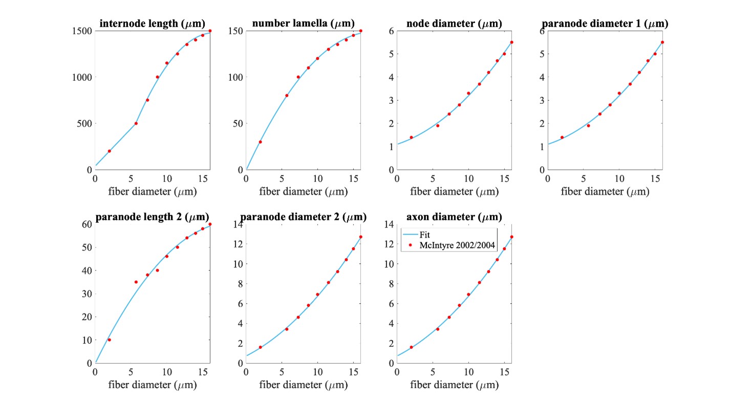
Piecewise polynomial fits to published MRG fiber parameters. Single quadratic fits were used for all parameters except for internode length, which has a linear fit below 5.643 µm (using MRG data at 2 and 5.7 µm) and a single quadratic fit at diameters greater than or equal to 5.643 µm (using MRG data >= 5.7 µm); 5.643 µm is the fiber diameter at which the linear and quadratic fits intersected. The fiber diameter is the diameter of the myelin. “Paranode 1” is the MYSA section, “paranode 2” is the FLUT section, and “internode” is the STIN section. The axon diameter is the same for the node of Ranvier and MYSA (“node diameter”), as well as for the FLUT and STIN (“axon diameter”). The node and MYSA lengths are fixed at 1 and 3 μm, respectively, for all fiber diameters.

We compared fiber activation thresholds between the originally published MRG fiber models and the interpolated MRG ultrastructure (evaluated at the original diameters) at a single location in a rat cervical vagus nerve stimulated with the bipolar Purdue cuff. Each fiber was placed at the centroid of the best-fit ellipse of the monofascicular nerve sample. The waveform was a single biphasic pulse using "BIPHASIC_PULSE_TRAIN_Q_BALANCED_UNEVEN_PW" with 100 µs for the first phase, 100 µs interphase (0 mA), and 400 µs for the second phase (cathodic/anodic at one contact and anodic/cathodic at the other contact). The thresholds between the originally published models and the interpolation of the MRG fiber diameters are compared in the image below. The threshold values were determined using a bisection search until the upper and lower bound stimulation amplitudes were within 1%.

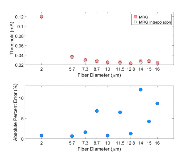
Comparison of thresholds between the originally published models and the interpolation of the MRG fiber diameters (evaluated at the original diameters). Thresholds are expected to vary between the originally published models and the interpolated fiber geometries given their slightly different ultrastructure parameters. Used original MRG thresholds as reference.

Small fiber MRG interpolated diameters - Version 1

The "FiberGeometry" mode "SMALL_MRG_INTERPOLATION" in Sim instructs the program to simulate a double cable structure for mammalian myelinated fibers for any diameter fiber between 1.011 µm and 16 µm. We redefined the geometric dimensions of myelinated fibers because the MRG geometries were not parameterized for small diameters <2 µm present in the rat cervical vagus nerve. We fit equations to ultrastructure parameter data from small fiber diameters in the literature (Figure A). We performed all linear or quadratic fits in MATLAB R2018a (‘fit’ function with ‘poly1’ or ‘poly2’ option). We subtracted the mean of the independent variables from each independent variable data point to ensure fit stability and avoid multicollinearity as well as to produce readily interpretable fit parameters. We weighted or transformed the dependent or independent variable to ensure nonnegative parameter values with means and uncertainties that tracked the data from the literature. Specifically, for FLUT length and internodal length, we performed weighted linear least squares regression (via the ‘Weight’ option of the ‘fit’ function) with weights equal to the inverse of the square of the FLUT length or internodal length, respectively, due to the observation that data uncertainty was proportional to the parameter value itself. For internodal axon diameter and nodal axon diameter, we performed linear least squares regression on the g-ratio (i.e., ratio of internodal axon diameter to myelin diameter) and on the ratio of the nodal axon diameter to the internodal axon diameter. For the number of myelin lamellae, we performed linear least squares regression on the natural log of the number of lamellae. The transformations and weighting are reflected in the final fit equations shown in Figure A.

Small myelinated fiber models that used the original MRG model ion channel conductances generated multiple action potentials per stimulus pulse. Therefore, we increased the maximum conductance of voltage-gated potassium ion channels (gkbar = 0.116 S/cm2) and decreased the maximum conductance of fast voltage-gated sodium ion channels (gnabar = 2.333 S/cm2) to obtain models that fired a single action potential per stimulus pulse. With the default combination of maximum conductance values (i.e., gnabar=3 S/cm^2 & gkbar=0.8 S/cm^2), multiple irregular action potentials occurred at some small fiber diameters (Figure B). Scaling gnabar and gkbar independently by 0 .33, 0.56, 0.78, 1.00, 1.22, 1.44, 1.67 and simulating all possible conductance combinations revealed that increasing the gnabar or decreasing gkbar could further increase firing or produce other unusual transmembrane potentials (Figure B). In contrast, decreasing the fast sodium channel’s maximum conductance or increasing the potassium channel’s maximum conductance could decrease multiple action potential firing. For all our analyses in the main text, we set gnabar to 2.333 S/cm^2 and gkbar to 0.116 S/cm^2 because the transmembrane potentials at those maximum conductances exhibited only a single action potential across all simulated axons (Figure C). We implemented the new small diameter MRG fiber model as described in [Peña et al., 2024].

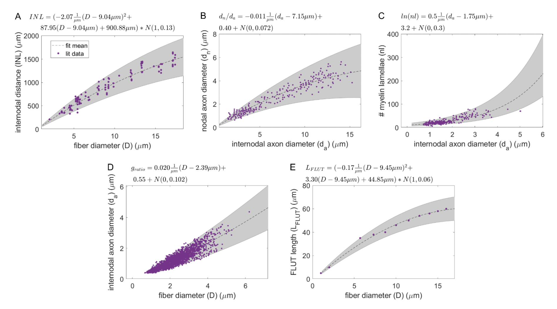
Figure A. Models of ultrastructure parameters for myelinated fibers (model equations denoted above each panel; Gaussian noise specified as N(mean, std)). Models were constructed via linear regression of ultrastructure parameters from the literature (yellow dots) to quantify the mean and variance of each parameter (black dotted line and gray shaded area). The gray areas represent the 95% confidence interval of the data variability. (A) Internodal length (INL) vs. fiber diameter (D) (fit to data from adult cat shown in Figure 3 of [Hursh, 1939]), with uncertainty modeled as a fraction of internodal length. The STIN length is calculated as the internodal length (panel A), minus the nodal length (fixed at 1 µm), minus twice the MYSA length (fixed at 3 µm), minus twice the FLUT length (panel E). (B) Ratio of nodal axon diameter (dn) to internodal axon diameter (da) (fit to data from Figures 3 & 4 of [Rydmark, 1981]). The nodal axon diameter is also equal to the MYSA axon diameter. (C) Number of myelin lamellae (nl) (fit to data from Figures 3A to 3C of [Friede and Samorajski, 1967]), with data log-transformed to exploit the discrete nature of the parameter via assumption of a Poisson distribution of noise. (D) Internodal axon diameter (fit to data from Figure 3 of [Friede and Samorajski, 1967] and Figure 3 (proximal and distal) from [Fazan et al., 1997]), which was transformed to g-ratio (ratio of internodal axon diameter to myelin diameter) for fitting. This parameter is also equal to the FLUT axon diameter. (E) FLUT length (LFLUT) (fit to data from [McIntyre et al., 2004, McIntyre et al., 2002]), with uncertainty modeled as a fraction of FLUT length.

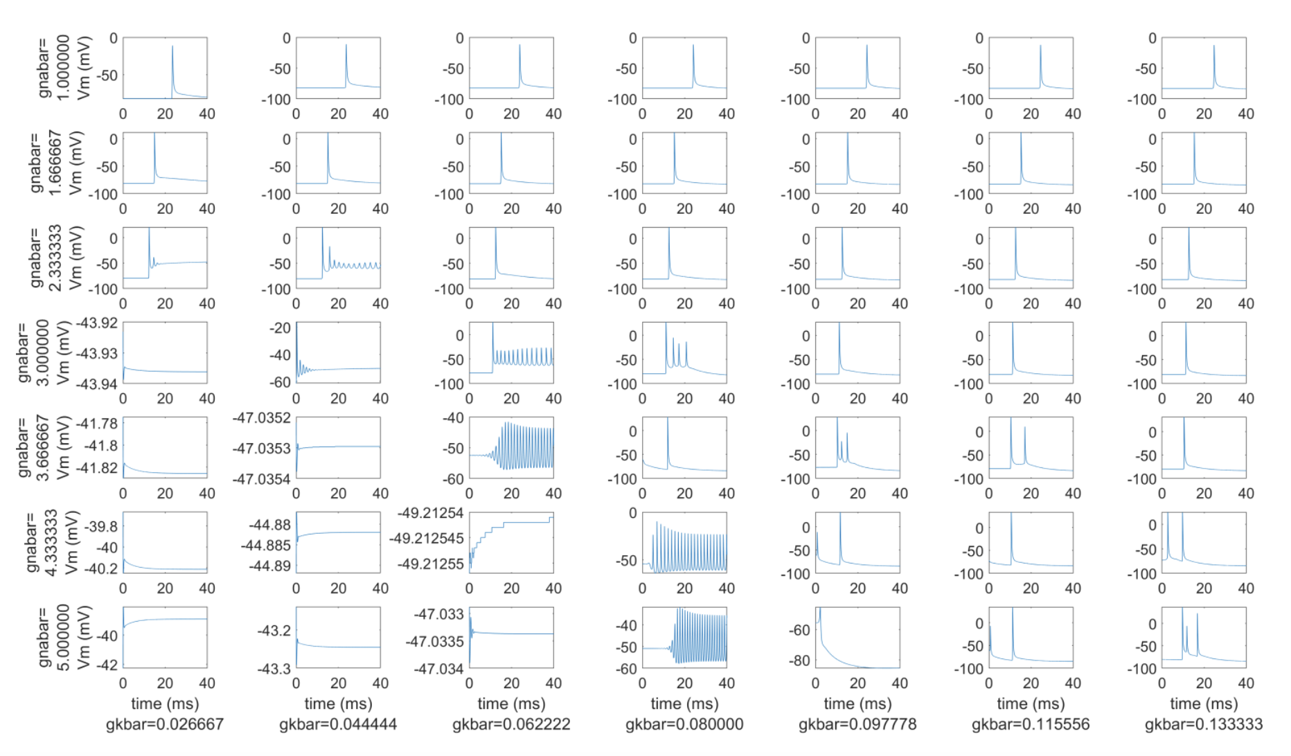
Figure B. Transmembrane potential traces at a single node of a 50 mm-long, 1.6 μm diameter myelinated fiber across a range of fast sodium channel maximum conductances (gnabar, in S/cm^2; row labels) and a range of maximum potassium channel conductance values (gkbar, in S/cm^2; column labels). The default conductances from (63) are gnabar=3 S/cm^2 and gkbar 0.8 S/cm^2 (center panel). We stimulated each axon with an intracellular stimulus pulse of 0.8 nA amplitude at the second node of Ranvier, and we recorded the transmembrane potential at the node closest to the 40 mm point along each axon.

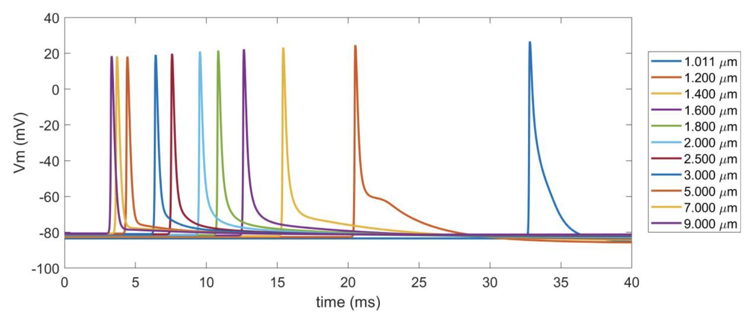
Figure C. Action potentials across myelinated fiber diameters with gnabar=2.333 S/cm^2 and gkbar=0.116 S/cm^2. The line colors are not unique across fiber diameters, but the latencies are ordered from fastest fiber (9 μm) to the slowest fiber (1.011 μm). We stimulated each axon with an intracellular stimulus pulse of 0.8 nA amplitude at the second node of Ranvier, and recorded the transmembrane potential at the node we closest to the 40 mm point along each axon.

Small fiber MRG interpolated diameters - Version 1

The "FiberGeometry" mode "SMALL_MRG_INTERPOLATION" in Sim instructs the program to simulate a double cable structure for mammalian myelinated fibers for any diameter fiber between 1.011 µm and 16 µm. We redefined the geometric dimensions of myelinated fibers because the MRG geometries were not parameterized for small diameters <2 µm present in the rat cervical vagus nerve. We fit equations to ultrastructure parameter data from small fiber diameters in the literature (Figure A). We performed all linear or quadratic fits in MATLAB R2018a (‘fit’ function with ‘poly1’ or ‘poly2’ option). We subtracted the mean of the independent variables from each independent variable data point to ensure fit stability and avoid multicollinearity as well as to produce readily interpretable fit parameters. We weighted or transformed the dependent or independent variable to ensure nonnegative parameter values with means and uncertainties that tracked the data from the literature. Specifically, for FLUT length and internodal length, we performed weighted linear least squares regression (via the ‘Weight’ option of the ‘fit’ function) with weights equal to the inverse of the square of the FLUT length or internodal length, respectively, due to the observation that data uncertainty was proportional to the parameter value itself. For internodal axon diameter and nodal axon diameter, we performed linear least squares regression on the g-ratio (i.e., ratio of internodal axon diameter to myelin diameter) and on the ratio of the nodal axon diameter to the internodal axon diameter. For the number of myelin lamellae, we performed linear least squares regression on the natural log of the number of lamellae. The transformations and weighting are reflected in the final fit equations shown in Figure A.

Small myelinated fiber models that used the original MRG model ion channel conductances generated multiple action potentials per stimulus pulse. Therefore, we increased the maximum conductance of voltage-gated potassium ion channels (gkbar = 0.116 S/cm2) and decreased the maximum conductance of fast voltage-gated sodium ion channels (gnabar = 2.333 S/cm2) to obtain models that fired a single action potential per stimulus pulse. With the default combination of maximum conductance values (i.e., gnabar=3 S/cm^2 & gkbar=0.8 S/cm^2), multiple irregular action potentials occurred at some small fiber diameters (Figure B). Scaling gnabar and gkbar independently by 0 .33, 0.56, 0.78, 1.00, 1.22, 1.44, 1.67 and simulating all possible conductance combinations revealed that increasing the gnabar or decreasing gkbar could further increase firing or produce other unusual transmembrane potentials (Figure B). In contrast, decreasing the fast sodium channel’s maximum conductance or increasing the potassium channel’s maximum conductance could decrease multiple action potential firing. For all our analyses in the main text, we set gnabar to 2.333 S/cm^2 and gkbar to 0.116 S/cm^2 because the transmembrane potentials at those maximum conductances exhibited only a single action potential across all simulated axons (Figure C). We implemented the new small diameter MRG fiber model as described in [Peña et al., 2024].

Figure A. Models of ultrastructure parameters for myelinated fibers (model equations denoted above each panel; Gaussian noise specified as N(mean, std)). Models were constructed via linear regression of ultrastructure parameters from the literature (yellow dots) to quantify the mean and variance of each parameter (black dotted line and gray shaded area). The gray areas represent the 95% confidence interval of the data variability. (A) Internodal length (INL) vs. fiber diameter (D) (fit to data from adult cat shown in Figure 3 of [Hursh, 1939]), with uncertainty modeled as a fraction of internodal length. The STIN length is calculated as the internodal length (panel A), minus the nodal length (fixed at 1 µm), minus twice the MYSA length (fixed at 3 µm), minus twice the FLUT length (panel E). (B) Ratio of nodal axon diameter (dn) to internodal axon diameter (da) (fit to data from Figures 3 & 4 of [Rydmark, 1981]). The nodal axon diameter is also equal to the MYSA axon diameter. (C) Number of myelin lamellae (nl) (fit to data from Figures 3A to 3C of [Friede and Samorajski, 1967]), with data log-transformed to exploit the discrete nature of the parameter via assumption of a Poisson distribution of noise. (D) Internodal axon diameter (fit to data from Figure 3 of [Friede and Samorajski, 1967] and Figure 3 (proximal and distal) from [Fazan et al., 1997]), which was transformed to g-ratio (ratio of internodal axon diameter to myelin diameter) for fitting. This parameter is also equal to the FLUT axon diameter. (E) FLUT length (LFLUT) (fit to data from [McIntyre et al., 2004, McIntyre et al., 2002]), with uncertainty modeled as a fraction of FLUT length.

Figure B. Transmembrane potential traces at a single node of a 50 mm-long, 1.6 μm diameter myelinated fiber across a range of fast sodium channel maximum conductances (gnabar, in S/cm^2; row labels) and a range of maximum potassium channel conductance values (gkbar, in S/cm^2; column labels). The default conductances from (63) are gnabar=3 S/cm^2 and gkbar 0.8 S/cm^2 (center panel). We stimulated each axon with an intracellular stimulus pulse of 0.8 nA amplitude at the second node of Ranvier, and we recorded the transmembrane potential at the node closest to the 40 mm point along each axon.

Figure C. Action potentials across myelinated fiber diameters with gnabar=2.333 S/cm^2 and gkbar=0.116 S/cm^2. The line colors are not unique across fiber diameters, but the latencies are ordered from fastest fiber (9 μm) to the slowest fiber (1.011 μm). We stimulated each axon with an intracellular stimulus pulse of 0.8 nA amplitude at the second node of Ranvier, and recorded the transmembrane potential at the node we closest to the 40 mm point along each axon.

Unmyelinated Fiber Models

The pipeline includes several unmyelinated (i.e., C-fiber) models [Rattay and Aberham, 1993, Sundt et al., 2015, Tigerholm et al., 2014]. Users should be aware of the "delta_zs" parameter that they are using in config/system/fiber_z.json, which controls the spatial discretization of the fiber (i.e., the length of each section). Note: ASCENT’s current functionality only supports the use of Tigerholm fiber model types.

Defining and assigning materials in COMSOL

Materials are defined in the COMSOL “Materials” node for each material “function” indicated in the “preset” cuff configuration file (i.e., cuff “insulator”, contact “conductor”, contact “recess”, and cuff “fill”) and nerve domain (i.e., endoneurium, perineurium, epineurium). Material properties for each function are assigned in Model’s “conductivities” JSON Object by either referencing materials in the default materials library (config/system/materials.json) by name, or with explicit definitions of a materials name and conductivity as a JSON Object (Material Parameters). See Add Material Definitions for code one how this happens.

Adding and assigning default material properties

Default material properties defined in config/system/materials.json are listed in Table A. To accommodate automation of frequency-dependent material properties (for a single frequency, i.e., sinusoid), parameters for material conductivity that are dependent on the stimulation frequency are calculated in Runner’s compute_electrical_parameters() method and saved to Model before the handoff() method is called. Our pipeline supports calculation of the frequency-dependent conductivity of the perineurium based on measurements from the frog sciatic nerve [Weerasuriya et al., 1984] using the rho_weerasuriya() method in the Python Waveform class. See Fig. 2 for identification of tissue types in a compound nerve cross-section (i.e., epineurium, perineurium, endoneurium).

Table A. Default material conductivities.

Material	Conductivity	References
silicone	10^-12 [S/m]	[Callister and Rethwisch, 2011]
platinum	9.43 ⨉ 10^6 [S/m]	[de Podesta, 1997]
endoneurium	{1/6, 1/6, 1/1.75} [S/m]	[Jr. and BeMent, 1965, Pelot et al., 2018]
epineurium	1/6.3 [S/m]	[Grill and Mortimer, 1994, Pelot et al., 2017, Stolinski, 1995]
muscle	{0.086, 0.086, 0.35} [S/m]	[Gielen et al., 1984]
fat	1/30 [S/m]	[Geddes and Baker, 1967]
encapsulation	1/6.3 [S/m]	[Grill and Mortimer, 1994]
saline	1.76 [S/m]	[Horch and Kipke, 2017]
perineurium	1/1149 [S/m]	[Pelot et al., 2018, Weerasuriya et al., 1984]

Definition of perineurium

The perineurium is a thin highly resistive layer of connective tissue and has a profound impact on thresholds of activation and block. Our previous modeling work demonstrates that representing the perineurium with a thin layer approximation (Rm = rho_peri_thk), rather than as a thinly meshed domain, reduces mesh complexity and is a reasonable approximation [Pelot et al., 2018]. Therefore, perineurium can be modeled with a thin layer approximation (except with “peanut” fascicles; see an example in Fig 2), termed “contact impedance” in COMSOL (if Model’s "use_ci" parameter is true (Model Parameters)), which relates the normal component of the current density through the surface \((\vec{n}\cdot\vec{J_{1}})\) to the drop in electric potentials \((V_{1}-V_{2})\) and the sheet resistance \((\rho_{s})\):

\[\vec{n}\cdot\vec{J_{1}}=\frac{1}{\rho_{s}}(V_{1}-V_{2})\]

The sheet resistance \((\rho_{s})\) is defined as the sheet thickness \((d_{s})\) divided by the material bulk conductivity \((\sigma_{s})\):

\[\rho_{s}=\frac{d_{s}}{\sigma_{s}}\]

Our previously published work quantified the relationship between fascicle diameter and perineurium thickness [Pelot et al., 2020] (Table A).

Table A. Previously published relationships between fascicle diameter and perineurium thickness.

Species	peri_thk: f(species, dfasc)	References
Rat	peri_thk = 0.01292*dfasc + 1.367 [um]	[Pelot et al., 2020]
Pig	peri_thk = 0.02547*dfasc + 3.440 [um]	[Pelot et al., 2020]
Human	peri_thk = 0.03702*dfasc + 10.50 [um]	[Pelot et al., 2020]

The “rho_perineurium” parameter in Model can take either of two modes:

• “RHO_WEERASURIYA”: The perineurium conductivity value changes with the frequency of electrical stimulation (for a single value, not a spectrum, defined in Model as “frequency”) and temperature (using a Q10 adjustment, defined in Model as “temperature”) based on measurements of frog sciatic perineurium [Pelot et al., 2018, Weerasuriya et al., 1984]. The equation is defined in src/core/Waveform.py in the rho_weerasuriya() method.

• “MANUAL”: Conductivity value assigned to the perineurium is as explicitly defined in either materials.json or Model without any corrections for temperature or frequency.