How to use ASCENT

Running the ASCENT Pipeline

See Running the Pipeline for instructions on how to run ASCENT. The first three stages of ASCENT are invoked by the command python run pipeline. This performs the necessary operations to prepare simulations of nerve stimulation. The final stage of ASCENT is invoked by the command python submit.py, which runs the simulations. After the simulations are run, the Query Class can be used to obtain the resultant data, and the Plotter Module can be used to visualize the results.

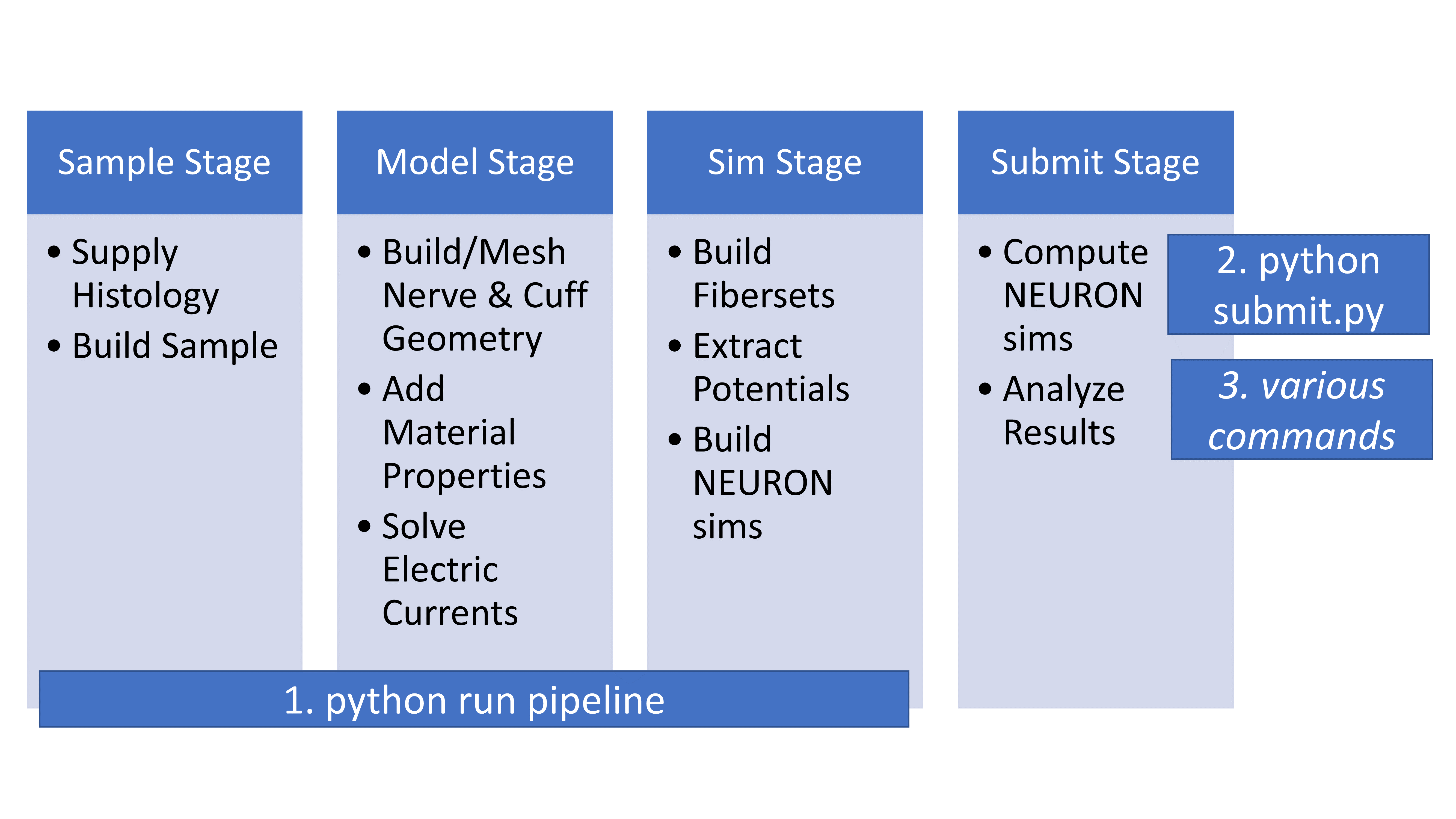
The stages of the ASCENT pipeline.

Submitting NEURON jobs

We provide scripts for the user to submit NEURON jobs in src/neuron/. The submit.py script takes the input of the Run configuration and submits a NEURON call for each independent fiber within an n_sim/. These scripts are called using similar syntax as pipeline.py: "./submit.<ext> <run indices>," where <run indices> is a space-separated list of integers. Note that these submission scripts expect to be called from a directory with the structure generated by Simulation.export_nsims() at the location defined by "ASCENT_NSIM_EXPORT_PATH" in env.json.

Cluster submissions

When using a high-performance computing cluster running SLURM:

1. Set your default parameters, particularly your partition (can be found in "config/system/slurm_params.json"). The partition you set here (default is “common” ) will apply to all submit.py runs.

2. submit.py will run in cluster mode if it detects that "sbatch" is an available command. To override this behavior manually, use Command-Line Arguments.

3. Many parameters which submit.py sources from JSON configuration files can be overridden with command line arguments. For more information, see Command-Line Arguments.

Other Scripts

We provide scripts to help users efficiently manage data created by ASCENT. Run all of these scripts from the directory to which you installed ASCENT (i.e., "ASCENT_PROJECT_PATH" as defined in config/system/env.json). For specific controls associated with each script, see Command Line Arguments.

scripts/import_n_sims.py

To import NEURON simulation outputs (e.g., thresholds, recordings of V_m) from your ASCENT_NSIM_EXPORT_PATH (i.e., <"ASCENT_NSIM_EXPORT_PATH" as defined in env.json>/n_sims/<concatenated indices as sample_model_sim_nsim>/data/outputs/) into the native file structure (see ASCENT Data Hierarchy, samples/<sample_index>/models/<model_index>/sims/<sim_index>/n_sims/<n_sim_index>/data/outputs/) run this script from your "ASCENT_PROJECT_PATH".

python run import_n_sims <list of run indices>

The script will load each listed Run configuration file from config/user/runs/<run_index>.json to determine for which Sample, Model(s), and Sim(s) to import the NEURON simulation data. This script will check for any missing thresholds and skip that import if any are found. Override this by passing the flag --force. To delete n_sim folders from your output directory after importing, pass the flag --delete-nsims. For more information, see Command-Line Arguments.

scripts/clean_samples.py

If you would like to remove all contents for a single sample (i.e., samples/<sample_index>/) EXCEPT a list of files (e.g., sample.json, model.json) or EXCEPT a certain file format (e.g., all files ending .mph), use this script. Run this script from your "ASCENT_PROJECT_PATH". Files to keep are specified within the python script.

python run clean_samples <list of sample indices>

scripts/tidy_samples.py

If you would like to remove ONLY CERTAIN FILES for a single sample (i.e., samples/<sample_index>/), use this script. This script is useful for removing logs, runtimes, special, and _.bat or _.sh scripts. Run this script from your "ASCENT_PROJECT_PATH". Files to remove are specified within the python script.

python run tidy_samples <list of sample indices>

scripts/build_from_input.py

You can organize your configuration files within the input directory. This will ensure repeatability for your runs by separating the input and output files for ASCENT. To use this configuration, create a directory /input/<input_name>, such as /input/tutorial. Place your image files in this directory as normal. Then create subfolders called /runs, /samples, /models, and /sims. Place your configuration JSON files in these folders respective to the configuration file type. In your /runs JSON files, instead of specifying integer indices for the sample, model, and sim files, use the file names from the subfolders. For example, the “sample” key in /input/runs/run_tutorial.json can have the value “sample_tutorial.json”, which will specify the file /input/<input_name>/samples/sample_tutorial.json as the sample configuration json for this run. Unique integers will be created for these configuration files in the appropriate ASCENT configuration directories, and a new rungroup called <input_name> will be created for the runs. Also see -i argument in pipeline.py.

python run build_from_input <input_name>

scripts/compare.py

This script will compare two folders in the /samples directory and saves a line-by-line difference to the /diff directory. This comparison may be helpful if you would like to verify that multiple runs differ by only the intended parameters.

The script iterates through the file tree and compares the files with Python’s filecmp module. Each folder with differing contents will have an analogous folder and file_compare.txt that summarizes the differences. The script then uses difflib to make line-by line comparisons for differing files, which are saved as <filename>_diff.txt. Finally, the script will load numerical values and compute the percent difference. These values are saved as <filename>_diff.dat in the /diff folder.

python run compare <sample_index> <sample_index>

Data analysis tools

Python Query class

The general usage of Query is as follows:

1. In the context of a Python script, the user specifies the search criteria (think of these as “keywords” that filter your data) in the form of a JSON configuration file (see query_criteria.json in Query Parameters).

2. These search criteria are used to construct a Query object, and the search for matching Sample, Model, and Sim configurations is performed using the method run().

3. The search results are in the form of a hierarchy of Sample, Model, and Sim indices, which can be accessed using the summary() method.

Using this “summary” of results, the user is then able to use various convenience methods provided by the Query class to build paths to arbitrary points in the data file structure as well as load saved Python objects (e.g., Sample and Simulation class instances).

The Query class’s initializer takes one argument: a dictionary in the appropriate structure for query criteria (Query Parameters) or a string value containing the path (relative to the pipeline repository root) to the desired JSON configuration with the criteria. Put concisely, a user may filter results either manually by using known indices or automatically by using parameters as they would be found in the main configuration files. It is extremely important to note that the Query class must be initialized with the working directory set to the root of the pipeline repository (i.e., sys.path.append(ASCENT_PROJECT_PATH) in your script). Failure to set the working directory correctly will break the initialization step of the Query class.

After initialization, the search can be performed by calling Query’s run() method. This method recursively dives into the data file structure of the pipeline searching for configurations (i.e., Sample, Model, and/or Sim) that satisfy query_criteria.json. Once run() has been called, the results can be fetched using the summary() accessor method. In addition, the user may pass in a file path to excel_output() to generate an Excel sheet summarizing the Query results. Finally, use the common_data_extraction(data_types=['threshold']) method to return a DataFrame of thresholds with identifying information. Other data_types are available with appropriate sim saving configurations:

• sfap

• threshold

• runtime

• activation

• istim

• time_gating

• time_vm

• space_gating

• space_vm

• aploctime

Query also has methods for accessing configurations and Python objects within the samples/ directory based on a list of Sample, Model, or Sim indices. The build_path() method returns the path of the configuration or object for the provided indices. Similarly, the get_config() and get_object() methods return the configuration dictionary or saved Python object (using the Pickle package), respectively, for a list of configuration indices. These tools allow for convenient looping through the data associated with search criteria.

Example uses of these Query convenience methods are included in examples/analysis/.

• plot_sample.py

• plot_fiberset.py

• plot_waveform.py

Specialized ASCENT plots

See Plotter Module for more info; example uses of this module are provided in examples/analysis.

Dose-response curves reflecting fiber diameters, types, and locations

In examples/analysis/ we provide a script, custom_fiber_dose_response_curve.py, that allows post-hoc analysis of fiber-specific diameters, types, and location data. The script accepts fiber data in the form of a .csv file and generates appropriate dose-response curves based on the data provided. The script was developed to allow for modeling interpretation of a large (>1000) amount of fibers, which are computationally resource intensive and unrealistic to model individually. Therefore, the script pulls data from and expands upon a base ASCENT simultation, which preemptively has gathered threshold results at equal fiber diameter intervals (e.g., every 1 um) along the full range of diameters within the nerve (i.e., within the input .csv file). We are able to do so based on the assumption that all fibers for a given diameter within a given fascicle have negligible differences between their thresholds Davis et al. (2023).

The csv file should have headers corresponding to the fiber locations and attributes, though only x and y locations are required. An example can be found in the /examples/tutorial/explicit_fibersets folder, which will work with the tutorial run of ASCENT.

Locations are xy-coordinates (in microns) placed on the nerve cross-section with respect to the bottom left corner of the input image. X and Y coordinates should be the first two columns of the .csv file (labelled with ‘x’ and ‘y’). The following columns can be any label or metric associated with the fiber, however fiber diameter columns must have the header “diameter”. All fiber locations should be placed within a fascicle’s inner boundary. Points that are outside of any inner perineurium boundary will be excluded from the dose-response curve and a warning will be printed to the terminal.

This script should be run after generating thresholds for a subset of your desired fibers through the normal ASCENT pipeline. For example, a sub-sampled simulation could contain fiber diameters spanning the range of your dataset in 2-um steps and placed only at the centroid of each fascicle in the sample cross section (see figure below). After running ASCENT normally with these parameters, edit the sample, model, and simulation indices as well as the location of the user-defined .csv file in the custom_fiber_dose_response_curve.py script. The script interpolates fiber thresholds at the new locations and diameters using quadratic. 1-D interpolation over fiber diameter. Plots generated from this script will show the dose-response curve of the fiber population defined in the .csv file.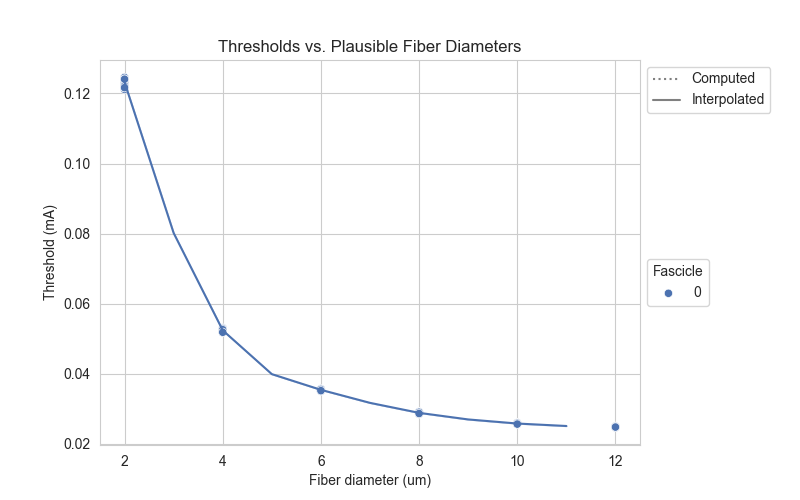

Video generation for NEURON state variables

In examples/analysis/ we provide a script, plot_video.py, that creates an animation of saved state variables as a function of space and time (e.g., transmembrane potentials, MRG gating parameters). The user can plot n_sim data saved in a data/output/ folder by referencing indices for Sample, Model, Sim, inner, fiber, and n_sim. The user may save the animation as either a *.mp4 or *.gif file to the data/output/ folder.

The plot_video.py script is useful for determining necessary simulation durations (e.g., the time required for an action potential to propagate the length of the fiber) to avoid running unnecessarily long simulations. Furthermore, the script is useful for observing onset response to kilohertz frequency block, which is important for determining the appropriate duration of time to allow for the fiber onset response to complete.

Users need to determine an appropriate number of points along the fiber to record state variables. Users have the option to either record state variables at all Nodes of Ranvier (myelinated fibers) or sections (unmyelinated fibers), or at discrete locations along the length of the fiber (Sim Parameters).