Python Classes

Warning

This page of our documentation is not actively updated, as we work on migrating code documentation to docstrings. Most of the information herein remains revelant, but please refer to the codebase for the most up to date structure.

Python classes for representing nerve morphology (Sample)

The nerve cross-section includes the outer nerve trace (if present; not required for monofascicular nerves) and, for each fascicle, either a single “inner” perineurium trace or both “inner” and “outer” perineurium traces. We provide automated control to correct for tissue shrinkage during histological processes [Boyd and Kalu, 1979] (Sample Parameters). Morphology metrics (e.g., nerve and fascicle(s) cross-sectional areas and centroids, major and minor axis lengths, and rotations of the best-fit ellipses) are automatically reported in Sample (Sample Parameters).

Trace

Trace is the core Python class for handling a list of points that define a closed loop for a tissue boundary in a nerve cross-section (see “Tissue Boundaries” in Fig 2). Trace has built-in functionality for transforming, reporting, displaying, saving, and performing calculations on its data contents and properties. Python classes Nerve, Fascicle, and Slide are all special instances or hierarchical collections of Trace.

A Trace requires inputs of a set of (x,y)-points that define a closed loop and an exceptions JSON configuration file. The z-points are assumed to be ‘0’. The Trace class already provides many built-in functionalities, but any further user-desired methods needed either to mutate or access nerve morphology should be added to the Trace class.

Trace uses the OpenCV [Bradski, 2000], Pyclipper [Chalton and others, 2015–], and Shapely [Gillies and others, 2007–] Python packages to support modifier methods (e.g., for performing transformations):

• scale(): Used to assign dimensional units to points and to correct for shrinkage of nerve tissues during processing of histology.

• rotate(): Performs a rigid rotational transformation of Trace about a point (positive angles are counter-clockwise and negative are clockwise).

• shift(): performs a 2D translational shift to Trace (in the (x,y)-plane, i.e., the sample cross-section).

• offset(): Offsets Trace’s boundary by a discrete distance from the existing Trace boundary (non-affine transformation in the (x,y)-plane, i.e., the sample cross-section).

• pymunk_poly(): Uses Pymunk to create a body with mass and inertia for a given Trace boundary (used in deform(), the fascicle repositioning method, from the Deformable class).

• pymunk_segments(): Uses Pymunk to create a static body for representing intermediate nerve boundaries (used in deform(), the fascicle repositioning method, from the Deformable class).

Trace also contains accessor methods:

• within(): Returns a Boolean indicating if a Trace is completely within another Trace.

• intersects(): Returns a Boolean indicating if a Trace is intersecting another Trace.

• centroid(): Returns the centroid of the best fit ellipse of Trace.

• area(): Returns the cross-sectional area of Trace.

• random_points(): Returns a random list of coordinates within the Trace (used to define axon locations within the Trace).

Lastly, Trace has a few utility methods:

• plot(): Plots the Trace using formatting options (i.e., using the plt.plot format, see Matplotlib documentation for details).

• deepcopy(): Fully copy an instance of Trace (i.e., copy data, not just a reference/pointer to original instance).

• write(): Writes the Trace data to the provided file format (currently, only COMSOL’s sectionwise format —ASCII with .txt extension containing column vectors for x- and y-coordinates—is supported).

Nerve

Nerve is the name of a special instance of Trace reserved for representing the outer nerve (epineurium) boundary. It functions as an alias for Trace. An instance of the Nerve class is created if the "NerveMode" in Sample (“nerve”) is “PRESENT” (Sample Parameters)”

Fascicle

Fascicle is a class that bundles together instance(s) of Trace to represent a single fascicle in a slide. Fascicle can be defined with either (1) an instance of Trace representing an outer perineurium trace and one or more instances of Trace representing inner perineurium traces, or (2) an inner perineurium trace that is subsequently scaled to make a virtual outer using Trace’s methods deepcopy() and offset() and the perineurium thickness defined by the "PerineuriumThicknessMode" in Sample ("ci_perineurium_thickness") (Sample Parameters). Upon instantiation, Fascicle automatically validates that each inner instance of Trace is fully within its outer instance of Trace and that no inner instance of Trace intersects another inner instance of Trace.

Fascicle contains methods for converting a binary mask image of segmented fascicles into instances of the Fascicle class. The method used depends on the contents of the binary image inputs to the pipeline as indicated by the "MaskInputMode" in Sample ("mask_input") (i.e., INNER_AND_OUTER_SEPARATE, INNER_AND_OUTER_COMPILED, or INNERS). For each of the mask-to-Fascicle conversion methods, the OpenCV Python package finds material boundaries and reports their nested hierarchy (i.e., which inner Traces are within which outer Traces, thereby associating each outer with one or more inners). The methods are expecting a maximum hierarchical level of 2: one level for inners and one level for outers.

• If separate binary images were provided containing contours for inners (i.tif) and outers (o.tif), then the "MaskInputMode" in Sample ("mask_input", Sample Parameters) is INNER_AND_OUTER_SEPARATE.

• If a single binary image was provided containing combined contours of inners and outers (c.tif), then the "MaskInputMode" in Sample ("mask_input", Sample Parameters) is INNER_AND_OUTER_COMPILED.

• If only a binary image was provided for contours of inners (i.tif), the "MaskInputMode" ("mask_input", Sample Parameters) in Sample is INNERS.

In all cases, the Fascicle class uses its to_list() method to generate the appropriate Traces. Additionally, Fascicle has a write() method which saves a Fascicle’s inner (one or many) and outer Traces to files that later serve as inputs for COMSOL to define material boundaries in a nerve cross-section (sectionwise file format , i.e., ASCII with .txt extension containing column vectors for x- and y-coordinates). Lastly, Fascicle has a morphology_data() method which uses Trace’s area() and ellipse() methods to return the area and the best-fit ellipse centroid, axes, and rotation of each outer and inner as a JSON Object to Sample (Sample Parameters).

Slide

The Slide class represents the morphology of a single transverse cross-section of a nerve sample (i.e., nerve and fascicle boundaries). An important convention of the pipeline is that the nerve is always translated such that its centroid (i.e., from best-fit ellipse) is at the origin (x,y,z) = (0,0,0) and then extruded in the positive (z)-direction in COMSOL. Slide allows operations such as translation and plotting to be performed on all Nerve and Fascicle Traces that define a sample collectively.

To create an instance of the Slide class, the following items must be defined:

• A list of instance(s) of the Fascicle class.

• "NerveMode" from Sample (“nerve”) (i.e., PRESENT as in the case of nerves with epineurium (n.tif) or NOT_PRESENT otherwise, (Sample Parameters)).

• An instance of the Nerve class if "NerveMode" is PRESENT.

• A Boolean for whether to reposition fascicles within the nerve from "ReshapeNerveMode" in Sample (Sample Parameters).

• A list of exceptions.

The Slide class validates, manipulates, and writes its contents.

• In Slide’s validation() method, Slide returns a Boolean indicating if its Fascicles and Nerve Traces are overlapping or too close to one another (based on the minimum fascicle separation parameter in Sample).

• In Slide’s smooth_traces() method, Slide applies a smooth operation to each Trace in the slide, leveraging the offset method, and applying smoothing based on smoothing parameters. defined in Sample (Sample Parameters).

• In Slide’s move_center() method, Slide repositions its contents about a central coordinate using Trace’s shift() method available to both the Nerve and Fascicle classes (by convention, in ASCENT this is (x,y) = (0,0)).

• In Slide’s reshaped_nerve() method, Slide returns the deformed boundary of Nerve based on the "ReshapeNerveMode" in Sample ("reshape_nerve", (Sample Parameters)) (e.g., CIRCLE).

• Using the methods of Nerve and Fascicle, which are both manifestations of Trace, Slide has its own methods plot(), scale(), and rotate().

• Slide has its own write() method which determines the file structure to which the Trace contours are saved to file in samples/<sample index>/slides/.

Note that the sample data hierarchy can contain more than a single Slide instance (the default being 0 as the cassette index and 0 as the section index, hence the 0/0 seen in ASCENT Data Hierarchy) even though the pipeline data processing assumes that only a single Slide exists. This will allow the current data hierarchy to be backwards compatible if multi-Slide samples are processed in the future.

Map

Map is a Python class used to keep track of the relationship of the longitudinal position of all Slide instances for a Sample class. At present, the pipeline only supports models of nerves with constant cross-sectional area, meaning only one Slide is used per FEM, but this class is implemented for future expansion of the pipeline to construct three-dimensional nerve models with varying cross-section (e.g., using serial histological sections). If only one slide is provided, Map is generated automatically, and the user should have little need to interact with this class.

Sample

The Sample class is initialized within Runner’s run() method by loading Sample and Run configurations (JSON Configuration Files). First, Sample’s build_file_structure() method creates directories in samples/ and populates them with the user’s file inputs from input/<NAME>/; the images are copied over for subsequent processing, as well as for convenience in creating summary figures. Sample then uses its populate() method to construct instances of Nerve and Fascicle in memory from the input sample morphology binary images (see Fascicle class above for details). Sample’s populate() method packages instances of Nerve and Fascicle(s) into an instance of Slide.

Sample’s get_factor() method obtains the ratio of microns/pixel for the input masks, either utilizing a scale bar image, or an explicit scale factor input depending on the user’s ScaleInputMode defined in Sample (Sample Parameters).

Sample’s scale() method is used to convert Trace points from pixel coordinates to coordinates with units of distance based either on the length of the horizontal scale bar as defined in Sample (micrometers) and the width of the scale bar (pixels) in the input binary image (s.tif), or on the explicitly specified scale ratio defined in Sample (Sample Parameters). If using a scale bar for scale input, it must be a perfectly horizontal line. Sample’s scale() method is also used within populate() to correct for shrinkage that may have occurred during the histological tissue processing. The percentage increase for shrinkage correction in the slide’s 2D geometry is stored as a parameter “shrinkage” in Sample (Sample Parameters). Additionally, Slide has a move_center() method which is used to center Slide about a point within populate(). Note that Sample is centered with the centroid of the best-fit ellipse of the outermost Trace (Nerve if "NerveMode" in Sample (“nerve”) is "PRESENT", outer Trace if "NerveMode" is "NOT_PRESENT", (Sample Parameters)) at the origin (0,0,0). Change in rotational or translational placement of the cuff around the nerve is accomplished by moving the cuff and keeping the nerve position fixed (Cuff Placement on the Nerve).

Sample’s im_preprocess() method performs preprocessing operations on the binary input masks based on the parameters given under preprocess in Sample (Sample Parameters).

Sample’s io_from_compiled() generates outers (o.tif) and inners (i.tif) from the (compiled) c.tif mask if "MaskInputMode" is INNER_AND_OUTER_COMPILED. These generated masks are then used in Fascicle’s to_list() method.

Sample’s generate_perineurium() method is used to generate the perineurium for fascicle inners in the case where "MaskInputMode" = INNERS. This leverages Trace’s offset() method, and fits the generated perineurium based on ci_perineurium_thickness defined in Sample (Sample Parameters).

Sample’s populate() method also manages operations for saving tissue boundaries of the Sample (Nerve and Fascicles) to CAD files (slides/#/#/sectionwise2d/) for input to COMSOL with Sample’s write() method.

Sample’s output_morphology_data() method collects sample morphology information (area, and the best-fit ellipse information: centroid, major axis, minor axis, and rotation) for each original Trace (i.e., Fascicle inners and outers, and Nerve) and saves the data under “Morphology” in Sample.

Lastly, since Sample inherits Saveable, Sample has access to the save() method which saves the Python object to file.

Deformable

If "DeformationMode" in Sample (“deform”) is set to NONE, then the Deformable class takes no action (Sample Parameters). However, if "DeformationMode" in Sample is set to PHYSICS, then Deformable’s deform() method simulates the change in nerve cross-section that occurs when a nerve is placed in a cuff electrode. Specifically, the outer boundary of a Slide’s Nerve mask is transformed into a user-defined final geometry based on the "ReshapeNerveMode" in Sample (i.e., CIRCLE) while maintaining the cross-sectional area. Meanwhile, the fascicles (i.e., outers) are repositioned within the new nerve cross-section in a physics-based way using Pymunk [Blomqvist, 2007], a 2D physics library, in which each fascicle is treated as rigid body with no elasticity as it is slowly “pushed” into place by both surrounding fascicles and the nerve boundary.

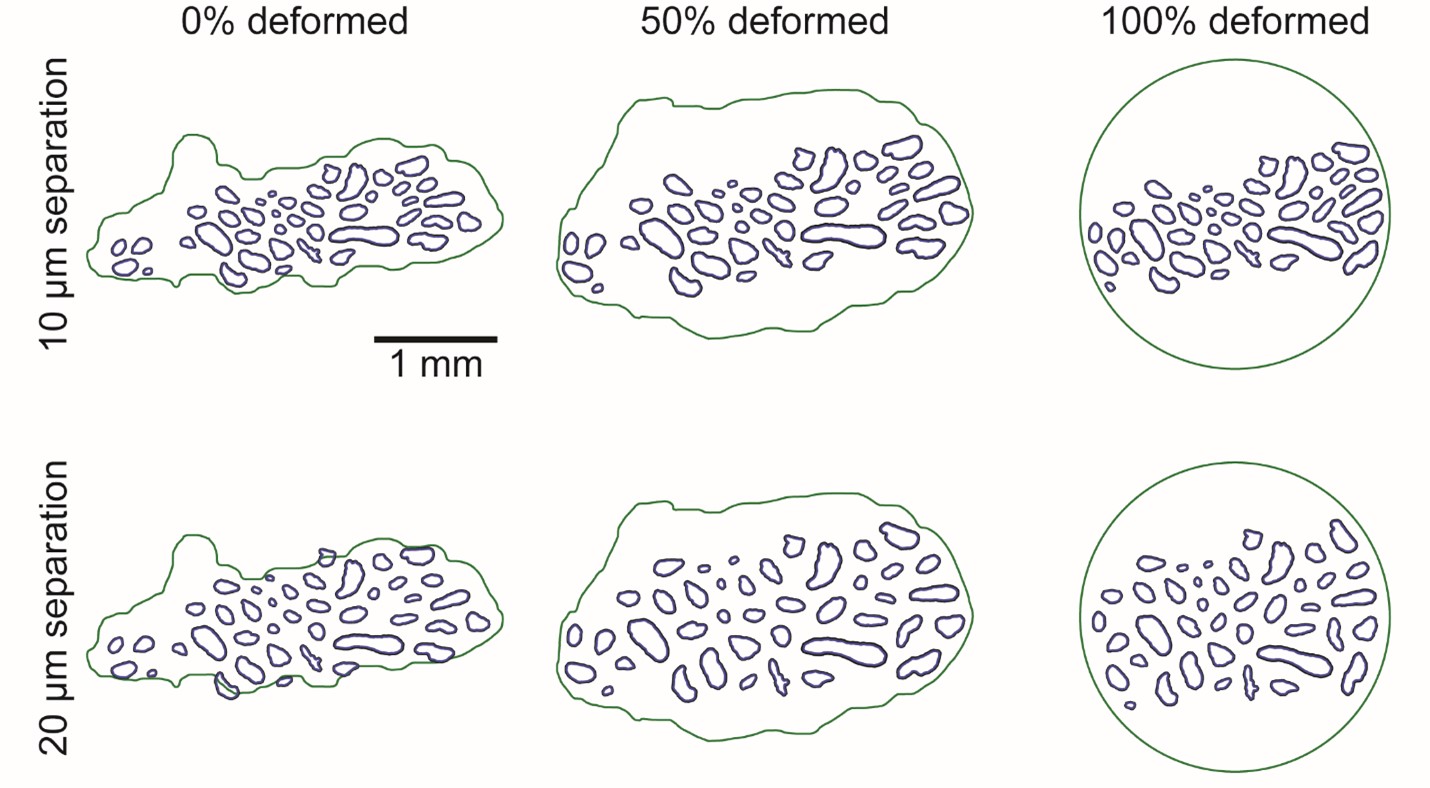
Snapshots at 0%, 50%, and 100% (left-to-right) of the deformation process powered by the pygame package [Shinners, 2011–]. The deformation process is shown for two minimum fascicle separation constraints: 10 µm (top row) and 20 µm (bottom row). The geometry at 0% deformation is shown after the fascicles have been spread out to the minimum separation constraint.

The deform() method updates the nerve boundary to intermediately-deformed nerve traces between the nerve’s "boundary_start" (i.e., the Trace’s profile in segmented image) and "boundary_end" (i.e., the Trace’s profile after accommodation to the cuff’s inner diameter, which is determined by the “ReshapeNerveMode” ("reshape_nerve", Sample Parameters) while the fascicle contents are allowed to rearrange in a physics-space. By default, all fascicles have the same “mass”, but their moment of inertia is calculated for each fascicle based on its geometry (see Trace’s pymunk_poly() method). Each fascicle is also assigned a “friction coefficient” of 0.5 as well as a “density” of 0.01. These measurements are mostly important as they relate to one another, not as absolute values. Importantly, we set the elasticity of all the fascicles to 0, so all kinetic energy is absorbed, and fascicles only move if they are directly pushed by another fascicle or by the nerve barrier. In Sample’s populate() method, the final fascicle locations and rotations returned by the deform() method are then applied to each fascicle using the Fascicle class’s shift() and rotate() methods.

Deformable’s convenience constructor, from_slide(), is automatically called in Sample’s populate() method, where a Slide is deformed to user specification. The from_slide() method takes three input arguments: The Slide object from which to construct the current Deformable object, the "ReshapeNerveMode" (e.g., CIRCLE, Sample Parameters), and the minimum distance between fascicles. If only inners are provided, virtual outers interact during nerve deformation to account for the thickness of the perineurium. Each inner’s perineurium thickness is defined by the "PerineuriumThicknessMode" in Sample ("ci_perineurium_thickness", Sample Parameters), which specifies the linear relationship between inner diameter and perineurium thickness defined in config/system/ci_peri_thickness.json (Contact Impedance). Deformable’s from_slide() method uses Deformable’s deform_steps() method to calculate the intermediately-deformed nerve traces between the boundary_start and the boundary_end, which contain the same number of points and maintain nerve cross-sectional area. The deform_steps() method maps points between boundary_start and boundary_end in the following manner. Starting from the two points where the major axis of the Nerve’s best-fit ellipse intersects boundary_start and boundary_end, the algorithm matches consecutive boundary_start and boundary_end points and calculates the vectors between all point pairs. The deform_steps() method then returns a list of intermediately-deformed nerve traces between the boundary_start and boundary_end by adding linearly-spaced portions of each point pair’s vector to boundary_start. Also note that by defining "deform_ratio" (value between 0 and 1) in Sample, the user can optionally indicate a partial deformation of the Nerve (Sample Parameters). In the case where "deform_ratio" is set to 0, minimum fascicle separation will still be enforced, but no changes to the nerve boundary will occur.

Enforcing a minimum fascicle separation that is extremely large (e.g., 20 µm) can cause inaccurate deformation, as fascicles may be unable to satisfy both minimum separation constraints and nerve boundary constraints.

To maintain a minimum distance between adjacent fascicles, the Deformable’s deform() method uses Trace’s offset() method to perform a non-affine scaling out of the fascicle boundaries by a fixed distance before defining the fascicles as rigid bodies in the pygame physics space. At regular intervals in physics simulation time, the nerve boundary is updated to the next Trace in the list of intermediately-deformed nerve traces created by deform_steps(). This number of Trace steps defaults to 36 but can be optionally set in Sample with the "morph_count" parameter by the user (Sample Parameters). It is important to note that too few Trace steps can result in fascicles lying outside the nerve during deformation, while too many Trace steps can be unnecessarily time intensive. We’ve set the default to 36 because it tends to minimize both aforementioned issues for all sample sizes and types that we have tested.

The user may also visualize nerve deformation by setting the "deform_animate" argument to true in sample.populate() (called in Runner’s run() method) (Sample Parameters). Visualizing sample deformation can be helpful for debugging but increases computational load and slows down the deformation process significantly. When performing deformation on many slides, we advise setting this flag to false.

Simulation

(Pre-Java)

The user is unlikely to interface directly with Simulation’s resolve_factors() method as it operates behind the scenes. The method searches through Sim for lists of parameters within the “fibers” and “waveform” JSON Objects until the indicated number of dimensions (“n_dimensions” parameter in Sim, which is a handshake to prevent erroneous generation of NEURON simulations) has been reached. The parameters over which the user has indicated to sweep in Sim are saved to the Simulation class as a dictionary named “factors” with the path to each parameter in Sim.

The required parameters to define each type of waveform are in Sim Parameters. The Python Waveform class is configured with Sim, which contains all parameters that define the Waveform. Since FEMs may have frequency-dependent conductivities, the parameter for frequency of stimulation is optionally defined in Model (for frequency-dependent material conductivities), but the pulse repetition frequency is defined in Sim as "pulse_repetition_freq". The write_waveforms() method instantiates a Python Waveform class for each "wave_set" (i.e., one combination of stimulation parameters).

(Post-Java)

The unique combinations of Sim parameters are found with a Cartesian product from the listed values for individual parameters in Sim: Waveforms ⨉ Src*weights ⨉ Fibersets. The pipeline manages the indexing of simulations. For ease of debugging and inspection, into each n_sim/ directory we copy in a modified “reduced” version of Sim with any lists of parameters replaced by the single list element value investigated in the particular n_sim/ directory.

The Simulation class loops over Model and Sim as listed in Run and loads the Python "sim.obj" object saved in each simulation directory (sims/\<sim index\>/) prior to Python’s handoff() to Java. Using the Python object for the simulation loaded into memory, the Simulation class’s method build_n_sims() loops over the master_product_index (i.e., waveforms ⨉ (src*weights ⨉ fibersets)). For each master_product_index, the program creates the n_sim file structure (sims/<sim index>/n_sims/<n_sim index>/data/inputs/ and sims/<sim index>/n_sims/<n_sim index>/data/outputs/). Corresponding to the n_sim’s master_product_index, files are copied into the n_sim directory for a “reduced” Sim, stimulation waveform, and fiber potentials. Additionally, the program writes a HOC file (i.e., "launch.hoc") containing parameters for and a call to our Wrapper.hoc file using the Python HocWriter class.

To conveniently submit the n_sim directories to a computer cluster, we created methods within Simulation named export_n_sims(), export_run(), and export_neuron_files(). The method export_n_sims() copies n_sims from our native hierarchical file structure to a target directory as defined in the system env.json config file by the value for the "ASCENT_NSIM_EXPORT_PATH" key. Within the target directory, a directory named n_sims/ contains all n_sims. Each n_sim is renamed corresponding to its sample, model, sim, and master_product_index (<sample_index>_<model_index>_<sim_index>_<master_product_index>) and is therefore unique. Analogously, export_run() creates a copy of Run within the target directory in a directory named runs/. Lastly, export_neuron_files() is used to create a copy of the NEURON *.hoc and *.mod files in the target directory in directories named "HOC_Files" and "MOD_Files", respectively.

Fiberset

Runner’s run() method first loads JSON configuration files for Sample, Model, and Sim into memory and instantiates a Python Sample class. The Sample instance produces two-dimensional CAD files that define nerve and fascicle tissue boundaries in COMSOL from the input binary masks. The run() method also instantiates Python Simulation classes using the Model and Sim configurations to define the coordinates of “fibersets” where “potentials” are sampled in COMSOL to be applied extracellularly in NEURON and to define the current amplitude versus time stimulation waveform used in NEURON (“waveforms”). The Simulation class is unique in that it performs operations both before and after the program performs a handoff to Java for COMSOL operations. Before the handoff to Java, each Simulation writes fibersets/ and waveforms/ to file, and after the Java operations are complete, each Simulation builds folders (i.e., n_sims/), each containing NEURON code and input data for simulating fiber responses for a single Sample, Model, fiberset, waveform, and contact weighting. Each instance of the Simulation class is saved as a Python object using Saveable (Python Utility Classes, which is used for resuming operations after the handoff() method to Java is completed.

Within the write_fibers() method of the Python Simulation class, the Python Fiberset class is instantiated with an instance of the Python Sample class, Model, and Sim. Fiberset’s generate() method creates a set of (x,y,z)-coordinates for each Fiberset defined in Sim. The (x,y)-coordinates in the nerve cross-section and z-coordinates along the length of the nerve are saved in fibersets/.

Fiberset’s method _generate_xy() (first character being an underscore indicates intended for use only by the Fiberset class) defines the coordinates of simulated fibers in the cross-section of the nerve according to the "xy_parameters" JSON Object in Sim (Sim Parameters). The pipeline defines (x,y)-coordinates of the fibers in the nerve cross-section according to the user’s selection of sampling rules (CENTROID, UNIFORM_DENSITY, UNIFORM_COUNT, and WHEEL); the pre-defined modes for defining fiber locations are easily expandable. To add a new mode for defining (x,y)-coordinates, the user must add a "FiberXYMode" in src/utils/enums.py (Enums) and add an IF statement code block in _generate_xy() containing the operations for constructing “points” (List[Tuple[float]]). The user must add the parameters to define how fibers are placed in the nerve within the "xy_parameters" JSON Object in Sim. In Sim, the user may control the “plot” parameter (Boolean) in the “fibers” JSON Object to create a figure of fiber (x,y)-coordinates on the slide. Alternatively, the user may plot a Fibserset using the plot_fiberset.py script (Python Morphology Classes).

Fiberset’s private method _generate_z() defines the coordinates of the compartments of simulated fibers along the length of the nerve based on global parameters in config/system/fiber_z.json and simulation-specific parameters in the "fibers" JSON Object in Sim (i.e., "mode", "diameter", "min", "max", and "offset").

Python utility classes

Enums

In the Python portions of the pipeline we use Enums which are “… a set of symbolic names (members) bound to unique, constant values. Within an enumeration, the members can be compared by identity, and the enumeration itself can be iterated over.” Enums improve code readability and are useful when a parameter can only assume one value from a set of possible values.

We store our Enums in src/utils/enums.py. While programming in Python, Enums are used to make interfacing with our JSON parameter input and storage files easier. We recommend that as users expand upon ASCENT’s functionality that they continue to use Enums, adding to existing classes or creating new classes when appropriate.

Configurable

Configurable is inherited by other Python classes in the ASCENT pipeline to grant access to parameter and data configuration JSON files loaded to memory. Configurable is an important class for developers to understand because it is the mechanism by which instances of our Python classes inherit their properties from JSON configuration files (e.g., sample.json, model.json, sim.json, fiber_z.json). The Configurable class takes three input parameters:

SetupMode (from Enums)

Either NEW or OLD which determines if Configurable loads a new JSON (from file) or uses data that has already been created in Python memory as a dictionary or list, respectively.

ConfigKey (from Enums)

The ConfigKey indicates the choice of configuration data type and is also the name of the configuration JSON file (e.g., sample.json, model.json, sim.json, run.json, env.json).

Config

The Config input to Configurable can take one of three data types. If "SetupMode" is “OLD”, the value can be a dictionary or list of already loaded configuration data. If "SetupMode" is “NEW”, the value must be a string of the file path to the configuration file to be loaded into memory.

Example use of Configurable

When the Sample class is instantiated in Runner, it inherits functionality from Configurable (see Sample constructor __init__(self, exception_config: list) in src/core/sample.py).

After the Sample class is instantiated, the Sample configuration (index indicated in Run) is added to the Sample class with:

sample.add(SetupMode.OLD, Config.SAMPLE, all_configs[Config.SAMPLE.value][0])

With the Sample configuration available to the Sample class, the class can access the contents of the JSON dictionary. For example, in populate(), the Sample class gets the length of the scale bar from Sample with the following line:

self.search(Config.SAMPLE, ‘scale’, ‘scale_bar_length’)

Saveable

Saveable is a simple Python class that, when inherited by a Python class (e.g., Sample and Simulation) enables the class to save itself using Saveable’s save() method. Using pickle.dump(), the object is saved as a Python object to file at the location of the destination path, which is an input parameter to save().